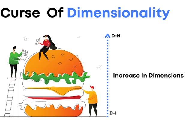
When dealing with high-dimensional data, there are a number of issues known as the “Curse of Dimensionality” in machine learning. The number of attributes or features in a dataset is referred to as the dimension of the dataset. High dimensional data refers to a dataset with a lot of attributes, typically on the order of 100 or more.
These days, this phenomenon is seen in a variety of industries, including machine learning, data analysis, and data mining. Theoretically, adding more information to the data can improve its quality, but in practice, adding dimensions only adds noise and redundancy to the analysis of the data.
Read More: What Is Boosting In Machine Learning?
Table of Contents
What Is Curse Of Dimensionality Machine Learning?
When working with high-dimensional data, there are a number of issues known as the “Curse of Dimensionality.” The number of attributes or features in a dataset is referred to as its dimension. High dimensional data refers to a dataset with many attributes, typically one hundred or more. High dimensional data presents a number of challenges when analyzing or visualizing the data to find patterns as well as when developing machine learning models. The difficulties related to training machine learning models due to high dimensional data are referred to as the ‘Curse of Dimensionality’
Domains Of Curse Of Dimensionality
Machine Learning is the most practical area where the direct impact of the curse of dimensionality can be observed.
The following is a list of the domains of the curse of dimension:
Anomaly Detection
To find unexpected items or events in the dataset, anomaly detection is used. Anomalies in high-dimensional data frequently display a striking number of attributes that are unrelated to their actual nature; some objects are more frequently found in neighbor lists than others.
Combinatorics
Every time there is a rise in the number of possible input combinations, the complexity soars and the curse of dimensionality manifests.
Machine Learning
In order to maintain the same level of performance in machine learning, a slight increase in dimensionality necessitates a significant increase in data volume. A phenomenon that manifests with high-dimensional data is the cause of the “curse of dimensionality,” or the problem with dimensions.

Feature Selection Tips
In feature selection techniques, the attributes are evaluated for value before being chosen or rejected. The following section discusses a few of the most popular feature selection methods.
Forward selection: One approach that can be used when creating multi-linear regression models from high dimensional data is one in which the regression model is initially constructed using only one attribute. later the remaining attributes are added one by one and tested for their worthiness using ‘Adjusted-R2’ values. If the Adjusted-R2 shows a noticeable improvement then the variable is retained else it is discarded.
Low Variance filter: With this method, attributes with a very low variance are disregarded after comparing the variance in the distribution of all the attributes in a dataset. The predictability of the model is not improved by attributes with low variance because they will be assumed to have a value that is nearly constant.
High Correlation filter: The pair-wise correlation between attributes is found using this method. When two attributes in a pair exhibit a high degree of correlation, one is dropped while the other is kept. The retained attribute captures the variation in the attribute that was eliminated.
Multicollinearity: If each attribute is regressed as a function of the others, we may see that the variability of some of the attributes is completely captured by the others. In some cases, a high correlation may not be found for pairs of attributes. This characteristic is known as multicollinearity, and Variance Inflation Factor (VIF) is a widely used method to identify multicollinearity. High VIF values, typically greater than 10, lead to the elimination of certain attributes.
Feature Ranking: The attributes can be ranked according to how important or helpful they are to the model’s predictability in decision tree models like CART. It may be possible to remove some of the lower-ranked variables from high-dimensional data in order to shrink those dimensions.
Impact Of Dimension Curse On Distance Functions
Any distance-based machine learning algorithms, such as KNN (k-Nearest Neighbor), tend to fall short when the number of dimensions in the data is very high. Dimensionality can therefore be seen as a “curse” in these algorithms.
Solutions To Curse Of Dimensionality
Using a different distance unit in a space vector is one method to lessen the effects of high dimensions. One could explore the use of cosine similarity to replace Cosine similarity may have less of an effect on data with higher dimensions compared to Euclidean distance. But the application of such a technique might also be tailored to the particular problem that needs to be solved.
Other methods:
Utilizing a reduction in dimensions could be used in other techniques. Among the methods that can be applied are:
1. choosing a forward feature: This approach entails selecting the most beneficial subset of features out of all available features.
2. Although PCA and t-SNE assist in reducing the number of features, they do not always preserve the class labels, which can make it challenging to interpret the results.
How To Deal With Effect Of Curse Of Dimensionality?
This was a general explanation of the dimensionality curse. In order to fully understand it, we will now get a little more technical. It can be described as follows in ML: as the number of features or dimensions “d” grows, the amount of data we require to generalize accurately grows exponentially. Data becomes sparse as dimensions rise, making it more challenging to generalize the model. More training data is necessary for the model to generalize more effectively.
1. Hughes Phenomenon
Let’s look at an illustration of this phenomenon once more. Assume that a dataset’s features are all binary. If the number of dimensions is 3, then there are 3 features then the total number of data points will be equal to 23 = 8. If there are 10 dimensions, then there are 10 features then the total number of data points will be equal to 210 = 1024. It is evident that as dimensionality rises, the number of data points also does so exponentially, indicating that dimensionality and the quantity of data needed to train a machine learning model are inversely correlated.
The Hughes phenomenon, which states that for a fixed size dataset, a machine learning model performs worse as dimensionality rises, is a very intriguing phenomenon.
2. Distance Functions (especially Euclidean Distance)
Consider a 1D world where n points are distributed at random between 0 and 1. In this world, point xi exists.
The two figures above show that the Euclidean distance between two points is very close to zero.
Now let me define two terms,
Dist_min (xi) = min{euc-dist(xi, xj} where xi is not equal to xj.
Dist_max (xi) = max{euc-dist(xi, xj} where xi is not equal to xj.
For 1D, 2D and 3D,
{[dist-max(xi) – dist-min(xi)] / dist-min(xi)} > 0
Taking the limit as d -> infinity, {[dist-max(xi) – dist-min(xi)] / dist-min(xi)} tends towards 0. You might be wondering what happens if this ratio tends to zero at this point.
We can see how those peaks are developing as the dimensions grow from the aforementioned figures. In the core of KNN, it works well if the pair of points are closer together in a cluster, but at higher dimensions, we can see the pair of points that are very close to each other reduces and we have many pairs of points having distances between 5 and 10 and 15 and more when d=100, and it only gets worse as the dimensions get bigger. Thus, we can be certain that KNN will disintegrate under these circumstances.
I will further explain it to you.
{[dist-max(xi) – dist-min(xi)] / dist-min(xi)}
The above ratio will only equal zero when the numerator equals zero, that is. dist-max and dist-min are equal, which means in higher dimensional spaces every pair of points are equally distant from every other pair of points. For instance, the separation between xi and xj is nearly equivalent to that between xi and xk. Every pair of points has this as their property.
Any machine learning model like KNN, which heavily relies on Euclidean distance, ceases to make logical sense whenever any pair of points in high-dimensional space are separated by the same amount as any other pair of points. As a result, KNN performs poorly as dimensionality rises. Although this was demonstrated in theory for n random points, it has also been demonstrated experimentally that KNN struggles in higher dimensional spaces. What then is the remedy?
The answer is very straightforward. Cosine-similarity should be used rather than Euclidean distance because it has less of an impact in higher dimensional spaces. For this reason, word-to-vec, TF-IDF, and other in-text problems are particularly challenging., cosine similarity is preferred because of high dimensional space.
All of these observations were made under the assumption that the distribution of the points is uniform and random, which is an important point to remember. So the next thought that occurs is what if the distribution of points is not even and random? We can approach this from a different perspective, i.e.
a) When points are dense and dimensionality is high, dimensionality has a significant impact.
b) The impact of dimensionality is minimal when points are sparse and dimensionality is high.
3. Overfitting And Underfitting
Overfitting and “d” have the following relationship:
d is directly proportional to overfitting i.e. as the dimensionality increases the chances of overfitting also increase.
Discussion of the issues that need to be resolved now.
a) Model-dependent methodology To choose the features that are most important for the prediction when there are many features, we can always perform forward feature selection.
b) In contrast to the above solution, which is classification-oriented, we can also use dimensionality reduction techniques like PCA and t-SNE, which do not use the class labels to determine the most pertinent features for the prediction.
Therefore, it’s crucial to remember that whenever you download a new dataset with a lot of features, you can reduce it using methods like PCA, t-SNE, or forward selection to make sure your model isn’t impacted by the curse of dimensionality.


